Ryan Kirgan's Blog

Named ranges are great. They allow the user to define a cell range with a single text-descriptor. For example, you could define the cell range of $A$1:$G$1 as the string “headings” and every time you wanted to refer to that cell range (in, say, a formula) you use the string “headings” instead.

I’ve alluded to them in Matching data in a table in Excel® using INDEX and MATCH (- a VLOOKUP alternative) and find named ranges invaluable for a number of reasons:

1. With appropriate “names” they can help explain what the range describes.
2. They (usu.) reduce the size of the formula(s).
3. They simplify reuse of the range.
4. By keeping the named range in a single location, if the range needs to be updated, it only needs to be changed once.
5. They reduce the chance of typographical errors when, particularly when used more than once.

The specific process of creating a named is slightly different in Excel® 2003 and Excel® 2007, however ostensibly you go about it the same way.

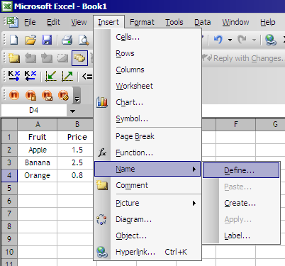
With Excel® 2003 you:

– Click on Define under the Name sub-menu of the Insert file menu.

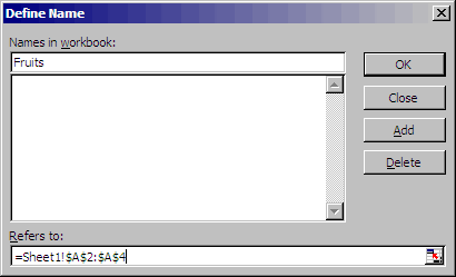
– Under Names in workbook: enter the name that describes the range.
– Under Refers to: enter the cell range that you want described by the “name”.

You can show that this works by using the INDEX function on the named range. For instance, the formula:

=INDEX(Fruits,1,1)

will return the value:

Apple

…and the formula:

=INDEX(Fruits,2,1)

will return the value:

Banana

A neat trick to get access to the named ranges when you are entering your formulas is to press F3. This will give you a list of the named ranges for you to pick from.

You can create ranges on individual columns, individual rows, or ranges that span many columns/rows.

For example, imagine you had a matrix of distances with origins as the row headings and destinations as the column headings:

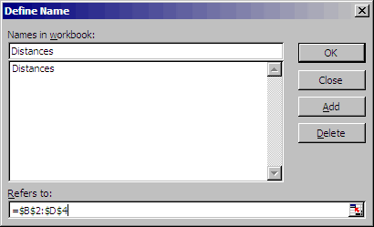
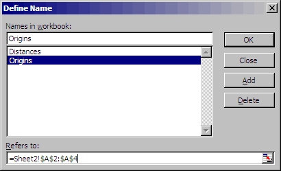
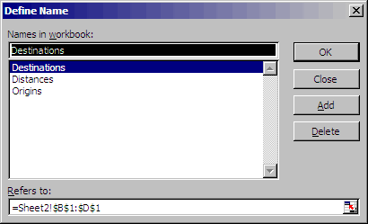
With the three (3) named ranges, “Origins”, “Destinations” and “Distances” defined thusly:

You could then find the distance between an origin and destination using the named ranges. You can use either INDEX & MATCH or SUMPRODUCT:

1. =INDEX(Distances,MATCH(“Sydney”,Origins,0),MATCH(“Melbourne”,Destinations,0))
2. =SUMPRODUCT(Distances*(Origins=”Sydney”)*(Destinations=”Melbourne”))

Both return 885. There are certainly more ways to do this…

Named ranges make it really clear what you are trying to search for – much like object oriented programming (OOP), using named ranges in this way make it easier for other people to understand what your code/formulas are trying to do. They reduce the chance of errors and reduce the time needed to replicate/propogate formulas.

Once you’ve mastered named ranges, you’ll find that there are many more application than what have been listed here. You might also find that there are limitations, least not, that you have to keep redefining your range every time you add more data (excluding inserting rows/columns in the middle of the range as it expands the cell range reference automatically.) If this is the case, you’re now ready for Dynamic Named Ranges: Creating Dynamic Named Ranges in Excel® using OFFSET & COUNTA

There are certainly aspects of the functions that I have omitted. I’d welcome any comments or criticism, so please feel free to add any comments. If you require further clarification on any part of this article, please leave a comment, or you can email me at: ryan@kirgs.com

Ryan Kirgan is from Sydney, Australia.