Skip to content

Creating Dynamic Named Ranges in Excel® using OFFSET & COUNTA

Following on from Creating Named Ranges in Excel®, this blog post describes how to create dynamic named ranges.

If you’re not familar with named ranges, I’d really suggest google searching “named ranges in excel” or read the post linked to above.

As mentioned many times on this site, named ranges are really useful, however there are situations where the data you need to reference is not in a static cell range – that is, the cell range is dynamic. To combat this, we can use the OFFSET and COUNTA functions.

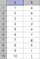
First, let’s look at COUNTA – it is a function that most Excel users would be familiar with. The COUNT function returns the number of numbers in a cell range. For instance:

1 to 10, a to j

1 to 10, a to j

Continue reading ›

Share
Tagged , , ,

Creating Named Ranges in Excel®

Named ranges are great. They allow the user to define a cell range with a single text-descriptor. For example, you could define the cell range of $A$1:$G$1 as the string “headings” and every time you wanted to refer to that cell range (in, say, a formula) you use the string “headings” instead.

I’ve alluded to them in Matching data in a table in Excel® using INDEX and MATCH (- a VLOOKUP alternative) and find named ranges invaluable for a number of reasons:

  1. With appropriate “names” they can help explain what the range describes.
  2. They (usu.) reduce the size of the formula(s).
  3. They simplify reuse of the range.
  4. By keeping the named range in a single location, if the range needs to be updated, it only needs to be changed once.
  5. They reduce the chance of typographical errors when, particularly when used more than once.

Continue reading ›

Share
Tagged ,

The weighing twelve (12) balls riddle – which one is a different weight?

This is a riddle that a friend (Carl “Chunky” Benson) put to me a few years back. A few A4 pages of scribblings and I had accounted for an “answer” for almost all possible outcomes (almost), however, I never arrived at a complete solution.

There’s every chance that I’m just hopeless at Maths, so prove me wrong people 🙂

Premise

  1. You have twelve (12) balls and a set of balance scales.
  2. One (1) of the balls is a different weight to the other eleven (11) balls.
  3. You are allowed to use the balance scales three (3) times.
  4. You need to determine which ball is the “odd one out” and whether it is heavier or lighter than the other balls.

Now these are balance scales I’m talking about. While a solution involving electronic scales would be effective, I don’t think it’s what the riddle’s architect had in mind 😉
Continue reading ›

Share
Tagged

Matching data in a table in Excel® using INDEX and MATCH – a VLOOKUP alternative

This post describes how you can use the INDEX() and MATCH() functions to look up data in a matrix.

Background to VLOOKUP()

Many users are familar with the VLOOKUP() (vertical lookup) function that simply looks up a value in the leading column of a table and returns the value in another specified column of the same table. The required parameters are:

VLOOKUP(Lookup_value,Table_array,Col_index_num,Range_lookup) where Range_lookup is optional.

For example:

With the data in the table below…

A B
1 Fruit Colour
2 Apple Red
3 Banana Yellow
4 Orange Orange (what else!)

…the formula

=VLOOKUP(“Banana”,$A$2:$B$4,2)

Result: Yellow

will search for “Banana” (1st parameter) in the leftmost column of the table ($A$2:$B$4) (2nd parameter) and return the value that is in the 2nd (3rd-parameter) column.

It should be noted that the 1st parameter (the value of which, here, is “Banana“) can also be a cell reference (e.g. $D$1) rather than statically entered into the result cell formula.
Continue reading ›

Share
Tagged